Axens Analyst
This tutorial page will guide you through the creation and deployment of a very simple soft sensor on Connect'In.
An Example of Soft Sensor Creation.
What is a Soft Sensor?
Soft sensors are used to predict response variables, which are difficult to measure, using the data of predictors that can be obtained relatively easier.
A soft sensor creates a new or replacement (twin) signal based on the calculations made by embedded algorithms that are trained on historical data.
Soft sensors are the combination of robust on-line sensor signals with mathematical models for deriving additional process information
What is Axens Analyst?
- Axens Analyst is a Connect'In plugin developed by Axens;
- It allows users to create machine learning models in a no-code environment;
- The choice of models range from regression to random forest;
- The created models can then be used as soft sensors.


Soft Sensor Example: What are you trying to predict?
The first question to ask yourself is what are you trying to predict?
Somes examples:
- Low frequency laboratory data;
- Unit performance prediction (yield, productivity or utility consumption).
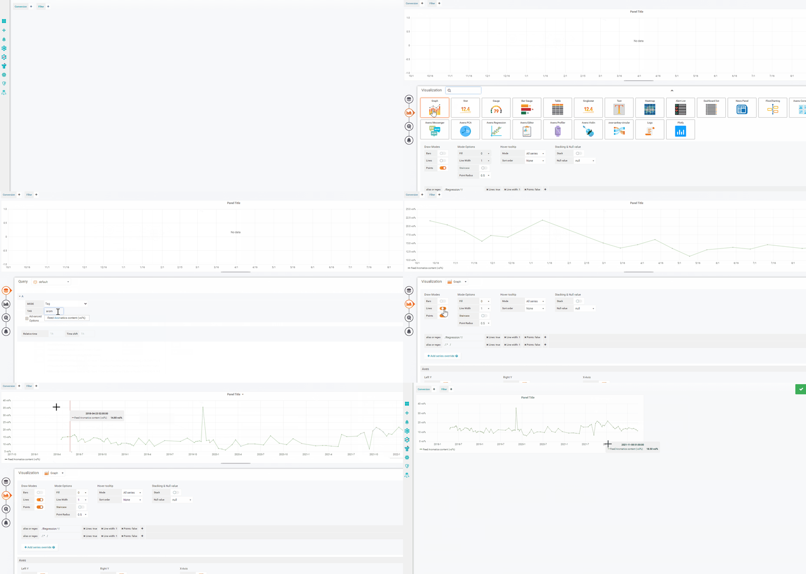
Whatever it is, you should plot it on a time series graph (refer to the basic tutorials to see how to do this) in order to look for outliers and abnormalities in the data.
In this example:
- We're looking to densify the laboratory analysis of aromatic content in the feed flowrate for semi regenerative reforming unit (SRR);
- The aromatic content is measured on a weekly basis;
- Our target is to have a daily value in order to improve the normalisation calculations.

Soft Sensor Example: Data Exploration
After plotting the target variable we need to start exploration the data that we have. Based on previous experience and process knowledge we already have an idea of the variables to investigate.
- Feed density - measured every day;
- Feed IBP & FBP - measued on a weekly basis.
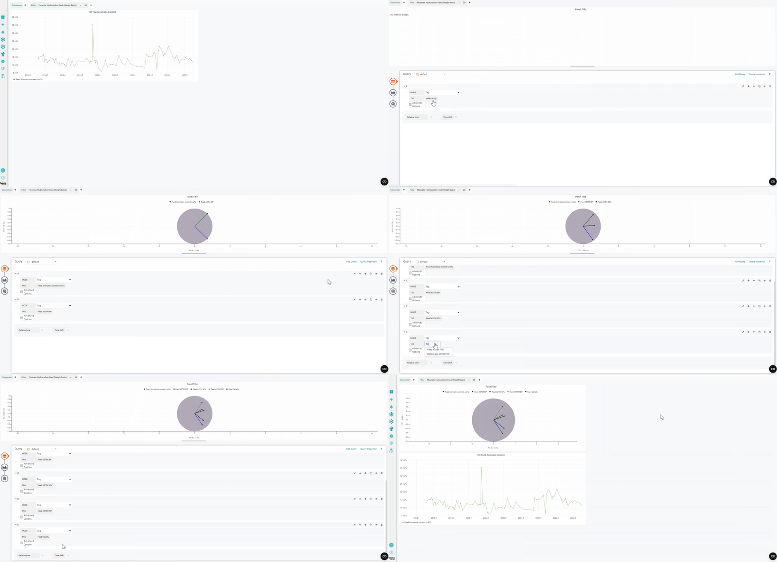
We filter by the unit feed flowrate > 30 t/h (> 70 % unit capacity) and use principle component analysis (PCA) to determine the optimum variables to use in the aromatic feed content prediction model.
From the PCA analysis we observe the following:
- Feed density is strongly postively correlated with the feed aromatic content compared to the distillation point measurements at the applied filter of > 30 t/h feed flowrate.
Soft Sensor Example
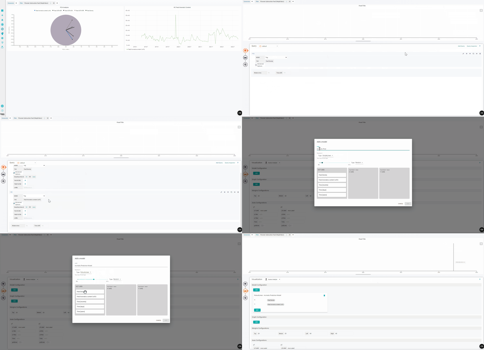
Now that we've identified a suitable variable (feed density) to use in our model let's try it out in the Axens Analyst.
The production of a model is a two part process:
1) Model creation;
2) Graph creation.
Both of which are done within the Axens Analyst Plugin

Soft Sensor Example: Model Creation
Soft Sensor Example: Model Graph Creation
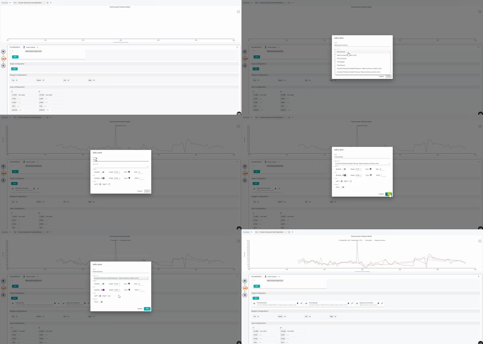
Model Performance
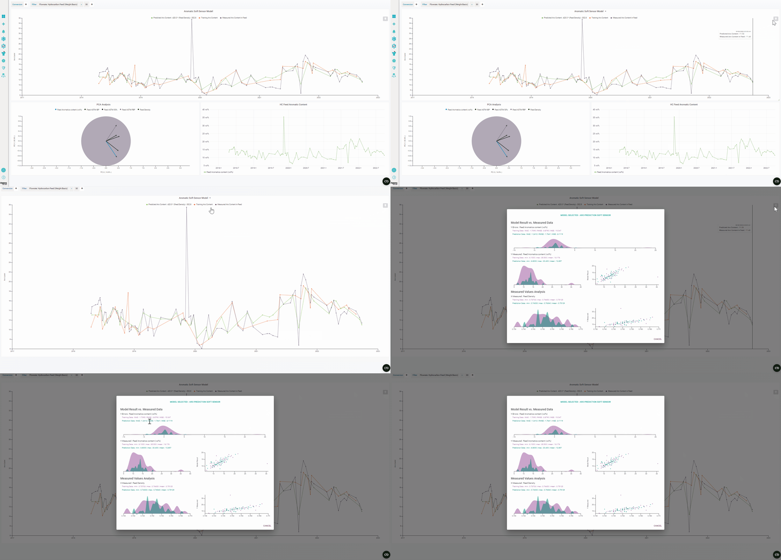
It is important to check the performance of our model using the KPIs calculated by the plugin.
- MAE - Average of absolute errors;
- MSE - The mean squared error (MSE) tells you how close a regression line is to a set of points. It does this by taking the distances from the points to the regression line (these distances are the “errors”) and squaring them;
- RMSE -Root Mean Square Error (RMSE) is the standard deviation of the residuals (prediction errors) .

Typically, the lower the better with the MSE, RMSE and MAE but be cautious that is not always the case!
How to Deploy my new Model?
So you will be thinking that's all well and good I have my equation:
Feed Aromatic Content = 420 * Feed Density - 302.8
But how do I use this in practice (compare it to the laboratory measurement) and display this on Connect'In??
To implement an equation in Connect'In you need to use a manual query as shown in the gif below. In manual queries the 'raw' tag name is used, hence the reference to Flow Config tag data management.

Predicted Aromatic Content (Yellow) vs. Measured Laboratory Values (Green)

Soft Sensor Completed!
Thank you for reading and don't hesitate to leave a comment on any techniques and actions done within this tutorial.
Goodluck for your future soft sensors using Axens Analyst!


